In this task, we will analyze text data. First, we will count how many times each word appears in our dataset. Then, we will create a word cloud to show which words are used most often. We will use the Tidy Text Mining website for guidance. We will also look at pairs of words (bigrams) to see common phrases and perform sentiment analysis to find out if the text is positive, negative, or neutral.

Load necessary libraries

# Load required packages for web scraping, text mining, and visualizing
library(rvest)
library(stringr)
library(tidytext)
library(tm)
library(wordcloud)
library(ggplot2)
library(tidyr)
library(dplyr)

Web Scraping

Specify the base URL of the website

base_url <- "https://www.tidytextmining.com"

Read the main webpage and extract links from the table of contents

webpage <- read_html(base_url)

toc_links <- webpage %>%
  html_nodes("nav a") %>%
  html_attr("href")

toc_links <- toc_links[grepl("^/", toc_links)]
page_urls <- paste0(base_url, toc_links)

Scrape content from each page

all_page_content <- list()

for (full_url in page_urls) {
  cat("Scraping content from:", full_url, "\n")
  
  webpage <- read_html(full_url)
  
  content_section <- html_nodes(webpage, css = "#content")
  content_text <- html_text(content_section)
  
  cleaned_content <- str_replace_all(content_text, "<script.*?</script>|<style.*?</style>", "")
  final_content <- str_squish(cleaned_content)
  
  all_page_content[[full_url]] <- final_content
}

## Scraping content from: https://www.tidytextmining.com/ 
## Scraping content from: https://www.tidytextmining.com/preface 
## Scraping content from: https://www.tidytextmining.com/tidytext 
## Scraping content from: https://www.tidytextmining.com/sentiment 
## Scraping content from: https://www.tidytextmining.com/tfidf 
## Scraping content from: https://www.tidytextmining.com/ngrams 
## Scraping content from: https://www.tidytextmining.com/dtm 
## Scraping content from: https://www.tidytextmining.com/topicmodeling 
## Scraping content from: https://www.tidytextmining.com/twitter 
## Scraping content from: https://www.tidytextmining.com/nasa 
## Scraping content from: https://www.tidytextmining.com/usenet 
## Scraping content from: https://www.tidytextmining.com/references

Combine all scraped content into a single data frame, and count the total words

all_content_df <- data.frame(page_url = names(all_page_content), content = unlist(all_page_content))

total_word_count <- sum(nchar(all_content_df$content) - nchar(gsub("\\s+", "", all_content_df$content)))

cat("Total word count:", total_word_count, "\n")

## Total word count: 39010

Data Cleaning

Clean the corpus and create a term-document matrix

corpus <- Corpus(VectorSource(all_content_df$content))
corpus <- tm_map(corpus, content_transformer(tolower))
corpus <- tm_map(corpus, removePunctuation)
corpus <- tm_map(corpus, removeNumbers)
corpus <- tm_map(corpus, removeWords, stopwords("en"))

tdm <- TermDocumentMatrix(corpus)
m <- as.matrix(tdm)

word_freq <- sort(rowSums(m), decreasing = TRUE)
valid_words <- grep("^[a-zA-Z]+$", names(word_freq), value = TRUE)

Visualization

Generate word cloud based on filtered word frequencies

wordcloud(words = valid_words, freq = word_freq[valid_words], min.freq = 10, 
          random.order = FALSE, colors = brewer.pal(8, "Dark2"))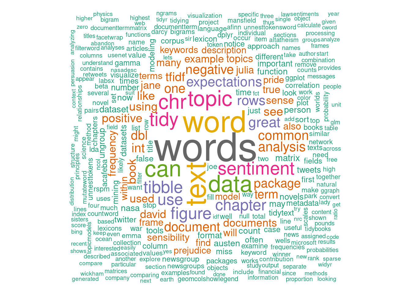

Create a bar plot for the top N words by frequency

top_n <- 10
top_words <- head(valid_words, n = top_n)
word_counts <- word_freq[top_words]

bar_data <- data.frame(word = top_words, frequency = word_counts)
bar_data <- bar_data[order(-bar_data$frequency), ]

ggplot(bar_data, aes(x = reorder(word, frequency), y = frequency)) +
  geom_bar(stat = "identity") +
  labs(title = paste("Top", top_n, "Words by Frequency"),
       x = "Word", y = "Frequency") +
  theme_minimal() +
  coord_flip()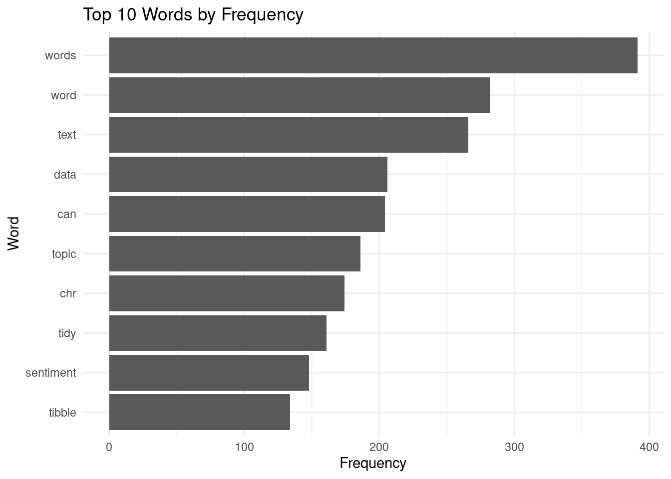

Analysis

Perform sentiment analysis and visualize results

corpus_tokens <- all_content_df %>%
  mutate(content = tolower(content)) %>%
  unnest_tokens(word, content) %>%
  anti_join(stop_words)

sentiment_scores <- corpus_tokens %>%
  inner_join(get_sentiments("bing"), by = "word") %>%
  count(word, sentiment) %>%
  spread(sentiment, n, fill = 0) %>%
  mutate(sentiment_score = positive - negative)

top_sentiment_words <- sentiment_scores %>%
  top_n(10, abs(sentiment_score)) %>%
  mutate(word = reorder(word, sentiment_score))

ggplot(top_sentiment_words, aes(x = word, y = sentiment_score, fill = sentiment_score > 0)) +
  geom_bar(stat = "identity", show.legend = FALSE) +
  scale_fill_manual(values = c("red", "green"), guide = FALSE) +
  labs(title = "Sentiment Analysis (Top 10 Words)",
       x = "Word", y = "Sentiment Score") +
  theme_minimal() +
  coord_flip()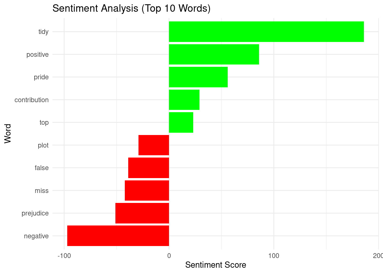

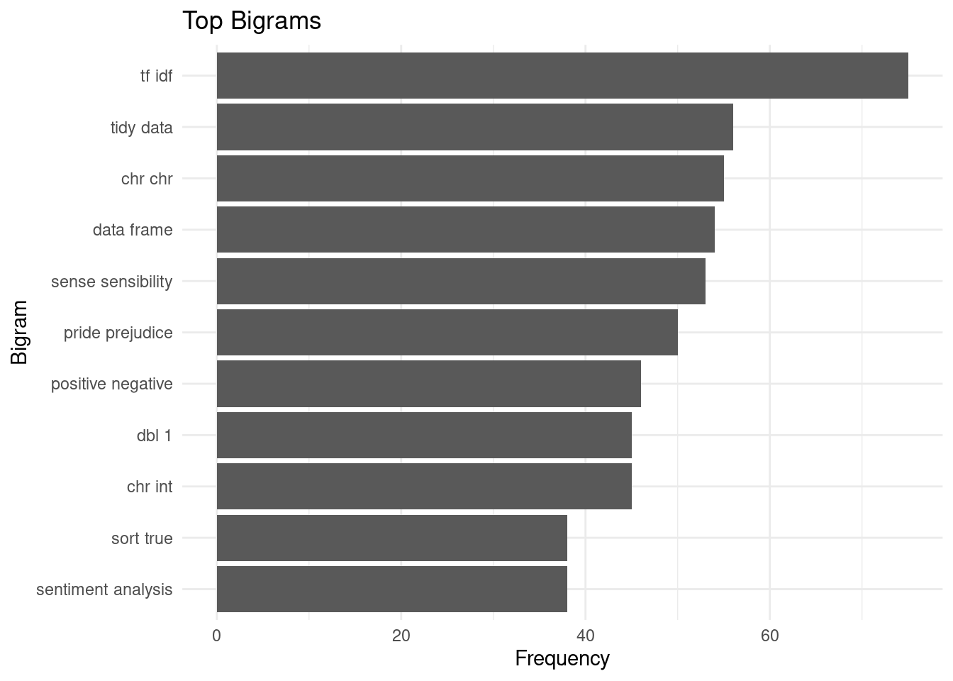
Extract bigrams from the corpus and visualize top bigrams

bigrams <- corpus_tokens %>%
  filter(!is.na(lead(word))) %>%
  mutate(bigram = paste(word, lead(word), sep = " ")) %>%
  count(bigram, sort = TRUE)

top_bigrams <- bigrams %>%
  filter(n > 10) %>%
  slice_max(order_by = n, n = 10)

ggplot(top_bigrams, aes(x = reorder(bigram, n), y = n)) +
  geom_col() +
  labs(title = "Top Bigrams",
       x = "Bigram", y = "Frequency") +
  theme_minimal() +
  coord_flip()

Word Count, Word Cloud, Bigram, and Sentiment